Week 1 Project Ideas

Tip

These are just suggested project ideas. You are free to come up with your own.

Project 1: Respiratory central pattern generator network in mammalian brainstem (Rubin et al. 2009)

XPPAUT Code link

Stereotypical rhythmic behaviours, both voluntary and involuntary, locomotion and breathing are generated by CPGs (Central Pattern Generators). These patterns are generated by interactions betweens the group of neurons (Nuclei or ganglion). Some special networks of these nuclei are capable of generating endogenous rhythms. These do not require rhythmic inputs but inherently generate patterned rhythmic patterns. Rubin et al 2009 models one such respiratory CPG located in the lower brain stem of mammalian brain. The motor pattern observed during normal breathing is considered to consist of three phases: a phase of inspiration, associated with phrenic motor activity producing lung inflation, and two expiratory phases: post-inspiration and late (stage 2) expiration. The simple things you can demonstrate with this model readily are :

(a) This tri-phasic response is shifted to a bi-phasic response when inputs from pons are removed.

(b) When more caudal inputs are reduced, the response shifts to a mono-phasic response.

(c) If you can control INap somehow (optogenetically or using blockers), it does not cause shift in the phase but changes its period.

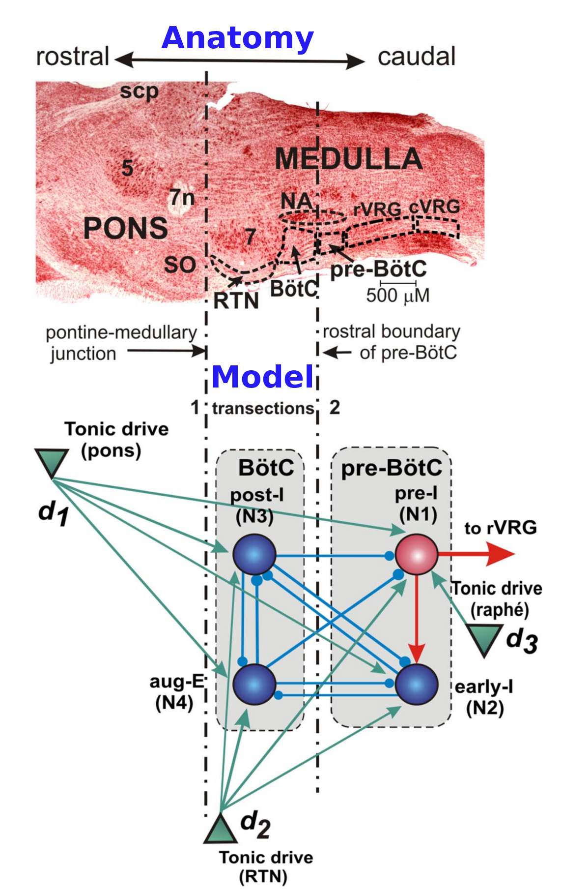
Citation-Multiple rhythmic states in a model of the respiratory central pattern generator doi:10.1152/jn.90958.2008

You can do many more things with this model. Abovementioned suggestions are just characterizations of the model. Some suggestions are as follows :

Bifurcation diagrams drawn using different bifurcation parameters can give you more clues about possibilities you can explore with this model. For example : You can investigate how more realistic patterns can be generated from controlling the drive to the CPGs. Let’s say you look at a paper like this. This measures complex-realistic breathing rhythms in mice. What are the ways to generate this kind of rhythm ? Are some inputs here voluntary (controlled by cerebral cortex) and involuntary ? (brainstem-intrinsic drive). How the breathing patterns are in behaviours where voluntary drive is extreme (high-singing, low or zero-sleeping/anesthesia) .

Project 2: Inverse stochastic resonance in Purkinje cells of cerebellum and its functional role in locally optimal information transfer (Buchin et al., 2016)

XPPAUT/MATLAB Code link

Purkinje neurons perform prominent computations in cerebellum through long dendritic arbours that go deep into cerebellar structures, unlike any other neuron type present in cerebellum. They have been shown to exhibit complex dynamics, display bistability and also display many interesting network phenomena like high frequency oscillations and travelling waves. Another special feature of these neurons is that they possess an excitability mechanism that allows them to be efficiently inhibited by a noise of a particular range of variance. This phenomenon is known as inverse stochastic resonance or ISR (for more details about this special phenomena and its other counterpart, ie, stochastic resonance refer to this) . Buchin et al 2016 present a simplified model of Purkinje neurons (adLIF experimentally fitted to purkinje neurons) . They and others have shown that a dynamical system with bistability is much needed to display ISR. What is interesting is that ISR allows purkinje neurons to efficiently perform many computations by operating in many regimes: ON and OFF (all-or-none toggle) or a filtering regime. Synaptic noise, or the noisy nature of synaptic firing (which we now know to be a feature and not a bug) allows purkinje cells to switch between these functional regimes. In essence, authors provide first evidence of functional significance of ISR . You can start with following things:

(a) Characterize the purkinje neuron wrt its excitability type, ie. type I or type II based on its Freq-Response curve. This gives us some clues about its dynamics. Compare the result of a ramping current input to your simulated neurons to an experimentally measured purkinje cell recording.

(b) The adLIF neuron was first formally described by Brete and Gerstner in 2003. Have a quick glimpse of their original paper and figure out which parameters control what aspect of the cell’s firing ? (adaptation, excitability type etc)

(c) Demonstrate that the Purkinje cells (simulated) show ISR for a particular variance band. How big is this band ? What parameters of the noise are important (mean,variance,duration etc) ? Does it matter what the distribution of the noise is ? (gaussian, poissonian,uniform, etc )

(d) Draw the bifurcation plot of the Purkinje neuron using XPPAUT. For what values of Iapp do you observe a Hopf bifurcation?

(e) Is there any relation between the values of variance for which the neuron shows ISR and where it shows the bifurcation ? Basically how is ISR related to the dynamics of the cell ?

(f) Something interesting I can suggest is as follows : change some intrinsic parameter, i.e., lets say adaptation rate or leak reversal or delta, a ,b. This now is not purkinje neuron anymore. Now redraw the bifurcation plot and again do (e). Where do the phenomena of ISR break down/modified/changed/become less stringent ?

(g) adLIF or Gerstner’s adLIF can exhibit both type I and type II excitability. Type I excitability: Neurons can fire at arbitrarily low frequencies just above threshold. Associated with a saddle-node bifurcation on an invariant circle (SNIC).Type II excitability: Neurons start firing at a finite frequency once threshold is crossed. Associated with a Hopf bifurcation. Now you must have characterized your neuron in (a). Does the other type exhibit ISR ? Why or why not ? (some hints might be in the bifurcation plot).

You can do many more things with this model. Abovementioned suggestions are just characterizations of the model. Some interesting broad questions to ask might be :

How ISR transforms short and long inputs in presence and absence of noise? What kind of computation does noise help with? Etc. . Another important thing to remember is : The function of cerebellar Purkinje cells is often considered in the context of adaptive filter models of the cerebellum.

Project 3: Binocular rivalry in a simple two-neuron model

(Original Source-link)

In binocular rivalry each eye views a different image but our perception alternates (time scale of seconds) between the images. Several existing models account for the oscillations by incorporating two neuronal populations that compete through mutual inhibition. A slow fatiguing mechanism, such as adaptation, mediates the back and forth switching of dominance. Here we study a simple ring-rate model. Let uj(t) be the ring rate of population j (j = 1, 2); aj(t) are the slow adaptation variables. The firing rates of the populations evolve in time according to the following set of ODEs:

duj/dt = -uj + f(-βui -γaj + Ij)

daj/dt = (uj -aj)/τa

with f(x) = 1/(1 + exp((θ − x)/k) and control parameter values: β = 0.9, γ = 0.5, I1= I2 = 0, τa = 10, θ = 0.2, k = 0.1.

1. Identify and describe the terms and parameters in the model (inhibition, external input, etc.)

2. Show that for β = 0.9 and I = 0.8 the model oscillates. Plot the time courses of u₁ and a₁ on the same axes (ordinate: -0.1 to 1.1, abscissa: 0 to 300), and describe the behavior (phases of dominance, suppression, etc). Overlay u₁ and u₂ on another plot and describe the trajectory. The underlying mechanism is bistability in the fast dynamics. Show it: think of a_j as slow; freeze them, say at 0.5 and look at u₁ and u₂ -nullclines.

3. Show that the model oscillates for a range of I -values; compute and plot the period, T vs I ; also plot max and min of u₁ vs I . According to Levelt’s Proposition 1 (LP1), based on psychophysical experiments, the oscillation period is expected to decrease as I increases. Does the model satisfy LP1?

4. Increase β (to 1.1) and compute the model’s behavior for 0 < I < 2.5; summarize it in a plot of amplitude vs I (bifurcation diagram); also, T vs I . Note and describe the new behavior (Winner-Take-All, WTA) for an intermediate range of I . Use some phase plane projections to demonstrate bistability in this WTA regime. For what I-range(s) is LP1 (more-or-less) satisfied or not satisfied?

5. Show that decreasing τₐ eliminates oscillations (why?) and leaves only the WTA regime.

6. Complete your response diagrams of amplitude of u₁ vs I by including the special uniform steady state (time independent, u₁ = u₂ , a₁ = a₂ ). Can you show analytically that it is monotonic?

7. Identify the kinds of bifurcations that occur as different solution states appear/disappear.

Project 4: Persistent spiking as a potential mechanism for supporting working memory (Ratte et al., 2018)

Github Repository

Most of the neurons use spikes to encode information. Some neurons can store information for short periods (seconds to minutes) by continuing to spike even after the stimulus is over. This mechanism has been speculated as a potential mechanism to enable working memory. This so-called “persistent” spiking occurs in many brain areas like medial prefrontal cortex (PFC),anterior cingulate cortex (ACC),Hippocampus,Amygdala and Entorhinal Cortex (EC). For example: Neurons of the prefrontal cortex exhibit persistent firing during the delay period of working memory tasks (Galloway, Evan M et al.). There is strong experimental evidence in PFC that Acetylcholine receptors (Muscarinic receptor) blockade compromises both working memory and persistent spiking activity. There are many possible mechanisms suggested for persistent spiking, recurrent connections and intrinsic neuronal bistability are a few to name. Intrinsic bistability has been linked to the calcium-activated, nonspecific cation current (ICAN), which has in turn, been linked to canonical transient receptor potential (TRPC) channels, especially TRPC5. These channels are gated by an influx of calcium.

Ratte et al. 2018 constructed a detailed model for ACC pyramidal neuron.

The simple things you can demonstrate with this model readily are :

a. Show that the ACC neurons show persistent firing even after the stimulus is off. Confirm whether it switches off the persistent firing after a long time ? If not, how can you switch off the persistent firing ?

b. You can draw the F-I curve of this neuron for different values of calcium activated nonspecific current (ICAN). See if this leads you to some interesting place ?

c. Use XPPAUT to draw a bifurcation plot for this neuron. You can choose different bifurcation parameters, depending upon what you find useful from the paper. What bifurcation does the system undergo and for what values of the bifurcation parameter?

You can do many more things with this model. Abovementioned suggestions are just characterizations of the model. Some interesting broad questions to ask might be :

You can do many things here. For example : look at this cartoon (link)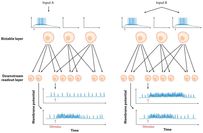

This cartoon is a simplified version of how a feed forward layer of bistable neurons that show persistent firing, can be used as a model to encode memory of a stimulus for a short time, even after the stimulus is gone. You can go this route or think of something more creative as well. What is the information content of stimulus in persistent firing ? You might have to look at the output of a group of ACC neurons.

Project 5: MCell

Astrocytic processes, especially perisynaptic astrocytic processes (PAPs), are thin (~100–300 nm diameter) and highly dynamic. These microdomains:

• Enwrap synapses

• Are rich in IP₃ receptors (IP₃Rs) on internal endoplasmic reticulum membranes

• Exhibit localized spontaneous Ca²⁺ signals called blips (single-channel events) and puffs (multi-channel events)

Experimental challenge: Due to their tiny size, these compartments are below the resolution of standard fluorescence microscopy, making it hard to determine:

• Molecular mechanisms

• Spatial organization

• Origin of spontaneous calcium signals

Particle-based spatial stochastic simulation is ideal for capturing:

• Spatial localization of receptors and signaling molecules

• Stochastic fluctuations in small volumes

• Colocalization-driven feedback mechanisms

This is where MCell comes in — a platform for realistic 3D, particle-based simulations of cell signalling at nanoscales.

Objectives

1. Replicate a spatial, stochastic model of spontaneous Ca²⁺ signaling via IP3Rs in fine astrocytic processes.

2. Quantify how IP₃R clustering (η) and calcium source colocalization radius (Rγ) affect:

   • Open probability of IP3 receptors

   • Amount of calcium in the cytosol

   • Proportion of blips vs puffs

All parameters and model details are provided in the paper below:.

Reference paper:

https://journals.plos.org/ploscompbiol/article?id=10.1371/journal.pcbi.1006795

“Simulation of calcium signaling in fine astrocytic processes: Effect of spatial properties on spontaneous activity”

Audrey Denizot, Misa Arizono, U. Valentin Nägerl, Hédi Soula, Hugues Berry

Project 6: MCell

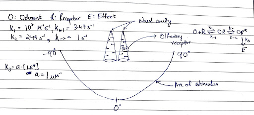
What is that smell? Where is it coming from? We have often found ourselves pondering these questions, regardless of the source of that smell. Interestingly, we are not alone in this inquiry; all complex organisms can ask the same. The olfactory system is arguably the oldest sensory system and is present across these organisms, allowing them to identify the source of an odorant by adjusting their nasal cavities or antennae and comparing the incoming signals.

In this project, you will design two identical conical nasal cavities using CellBlender and simulate the response of olfactory receptors to a diffusing odorant. By studying the dynamics of the receptors in the nasal cavity, can you determine the direction or angle of the odorant’s source? If so, please explain the underlying principle that enables the detection of the source’s direction or angle from the nasal cavity. Additionally, comment on the resolution of your system. Feel free to draw your own conclusions as well.

Feel free to play around with the rate constants.

You may use the following papers for further reference:

1. https://bpspubs.onlinelibrary.wiley.com/doi/pdfdirect/10.1002/prp2.311
2. https://pubs.acs.org/doi/10.1021/acs.jpcb.7b00486

Project 7: From spiking neurons to population dynamics — example on Wilson-Cowan model

Objective:

This project explores how the collective behavior of neural populations emerges from the interactions of individual spiking neurons. Using probabilistic methods inspired by Bressloff [1] and Benayoun et al. [2], the Wilson-Cowan equations [3,4] are derived from microscopic spiking dynamics. The analysis of this mean-field model explains key phenomena like bistability and oscillations in neural activity.

1. Mean-Field Approximation:

Let’s consider a network of stochastic binary neurons (0: quiescent state and 1: active state). Each neuron spiking (jump from 0 to 1) probability depends on its inputs from the other excitatory and inhibitory neurons. Considering the dynamics of the proportion of active neurons when the number of neurons tends to infinity, one can derive a mean field model which is nothing else than the famous WIlson-Cowan model.

2. Emergent Phenomena:

Analysing the limit system with dynamical system theory, one can find parameters generating interesting dynamics such as bistability and oscillations.

3. Numerical Exploration:

Simulations of the Wilson-Cowan model and its microscopic version enables one to visualize these phenomena, mapping out parameter regimes where bistability or oscillations occur.

4. Discussion:

What are the strengths and limitations of the mean-field approach? Consider when it breaks down (e.g., in small or highly correlated networks) and possible extensions to include noise or spatial structure.

Outcome:

The project highlights the interplay between theory (mean-field approximations) and phenomena (bistability, oscillations), offering intuition for how simplified models can capture complex neural behavior.

References:

[1] Bressloff, P. C. Metastable states and quasicycles in a stochastic Wilson-Cowan model of neuronal population dynamics. Physical Review E 82, 051903 (2010).

[2] Benayoun, M., Cowan, J. D., van Drongelen, W. & Wallace, E. Avalanches in a Stochastic Model of Spiking Neurons. PLoS Computational Biology 6, e1000846 (2010).

[3] Wilson, H. R. & Cowan, J. D. Excitatory and Inhibitory Interactions in Localized Populations of Model Neurons. Biophysical Journal 12, 1—24 (1972).

[4] Wilson, H. R. & Cowan, J. D. A mathematical theory of the functional dynamics of cortical and thalamic nervous tissue. Kybernetik 13, 55—80 (1973).

Project 8: On simple connectivity structure to generate oscillations

Objective:

This project explores how simple rules on the structure of connectivity can explain the emergence of oscillations. Starting with a simple linear system, one can derive a very simple rule due to Thomas [1]: if the number of inhibitory connections of the loops present in a linear network is odd, then oscillation will possibly emerge. This was proved by Snoussi [2] and Gouzé [3]. In a simple non-linear neural system, the threshold-linear model, there are some additional constraints on the weights [4].

1. The emergence of oscillations in linear systems:

The presence of oscillations can be determined by analysing the spectral properties of the Jacobian matrix of dynamical systems. Familiarising with this concept can be done through simple analytical computations as well as simulations.

2. Going beyond linearity:

The conditions for oscillations proposed in [4] for threshold-linear model can be tested numerically. What happens in more general networks with several loops as well as in spiking networks are very interesting open questions.

Outcome: Learn how fundamental connectivity rules (like inhibitory loops and excitation-inhibition balance) generate neural oscillations. By combining theory with simulations, students gain intuition for how network structure shapes dynamics — a key concept for understanding rhythms in biological and artificial neural circuits. The hands-on analysis reinforces how mathematical principles translate to observable phenomena in neuroscience.

References:

[1] Thomas R. 1980. On the relation between the logical structure of systems and their ability to generate multiple steady States or sustained Oscillations. Thomas R (Ed). Numerical Methods in the Study of Critical Phenomena. Springer. p. 180—193.

[2] Snoussi EH. 1998. Necessary conditions for multistationarity and stable periodicity. Journal of Biological Systems 06:3—9

[3] Gouzé JL. 1998. Positive and negative circuits in dynamical systems. Journal of Biological Systems 06:11—15.

[4] Zang, J., Liu, S., Helson, P. & Kumar, A. Structural constraints on the emergence of oscillations in multi-population neural networks. eLife 12, RP88777 (2024).

Project 9 : Role of dendritic sodium spikes in Neurons (Górski et al 2018)

Brian2 code.

Paper link

Dendrites can perform a variety of computations by nonlinear integration of synaptic inputs. For example: a single dendritic branch can perform coincidence detection, a computation crucial for phenomena like stereo-audition in the auditory system (review). It is speculated that an active, spiking dendrite can perform more subtle integration of synaptic inputs. Górski et al 2018 investigated the interaction between dendritic spikes and showed that with passive dendrites, an increase in correlation of synaptic input causes increase in firing rate. Whereas in active dendrites, the firing rate varies inversely with the correlation. (Inverse firing rate response). They constructed different models for soma (Gestner’s Adex and HH neuron) to show that active dendrites can perform a very different kind of computation than passive dendrites. You can take this idea further as much as you want.

Simple checks you can perform with this model are :

1. Show the positive correlation between synaptic activity and firingrate in point neurons (or ideally, construct a passive dendritewith a soma) and active-dendrite with inverse correlation.

2. Show that inverse correlation is affected by Na channel density(gNa). Check this, where does the system break on either side? Ifyou keep increasing gNa, will you still see inverse correlation?Is there an optimal window?. Investigate the values of gNa ofdendrite wrt somatic gNa. Are the values where the system breaksdown, a realistic value for gNa,

3. Authors claim that the absolute refractory period of spiking canaffect this inverse firing rate response. Confirm this claim. Howcan you rationalize the change in refractory period ofneuron/dendrite in real neurons ?

Many more interesting things can be done with this model. For starters, authors have shown this behaviour for cone-shaped dendrites. Is this property held by other shapes ? (cylinder, rectangular). How is the inverse correlation affected by the change in shape ? Which shape is affected the most by Na channel density? Check out the different shapes of dendrites present in brains. Which one of them is more suited for this kind of computation? Another thing that can be explored is, some dendrites show Ca++ spikes. It would be a serious challenge but if you must take it, check if this phenomenon is only exclusive to Na spikes? We will leave the rest of the exploration to the imagination of you all.

Project 10 : Detailed Gut mobility by pacemaker neurons (Barth et al 2017)

Brian2 code.

Paper link

Control of neuromodulation has been used as an effective therapy for many CNS and PNS diseases like Parkinson’s disease, Epilepsy and chronic pain. On the other hand, neuromodulatory control (by electrical stimulation of neurons controlling the Gut mobility) of the GI tract, which is in turn, stimulated by the enteric nervous system (ENS), has achieved relatively less success. Probably because the underlying mechanisms are poorly understood. Pathology of ENS can lead to compromised motility of the gut, causing functional GI disorders. These pathologies can be complicated to understand because of the intricate back and forth between smooth motor muscles and ENS circuitry. Barth et al 2017 constructed a detailed model of this Gut-Brain interaction. The model combines the gut mobility model with the neuronal network of ENS. Since it is difficult to record and interpret from ENS, this model gives a nice, testable way to understand the mechanism of peristalsis. Authors proposed that sinusoidal currents at 0.5 Hz applied to pacemakers of ICC were more effective at accelerating movements of the gut, as compared to square pulses of the same inputs. This was further validated by experiments in awake rats. So many things you can do with this model. For testing:

a. Authors suggest that the mobility of the pellet is sensitive tocharacteristics of the stimulus (sine, pulse, freq etc). Simulatethe model for all possible configurations described in the codeand figure out which stimulation has the maximum acceleration.

b. Authors investigated AHP channels in sensory neurons and their rolein gut mobility. You can recheck that as well. First, simulate theisolated Sensory cells with and without AHP and check what are thedifferences. Draw a F-I curve for sensory cells with and withoutAHP. Are there any differences?

c. How is mobility affected by pellet size? Do all sizes of pellet havemax mobility for sine wave stimulation of 0.5 Hz as suggested byauthors?

After this check, many more interesting things can be done with this model. For example: Is there a freq regime where pulses work better than sine waves? Is sine stimulation the best way to simulate the sensory neurons for maximum mobility? Try different stimulation (oscillatory and non oscillatory like poissonian) and check what happens to the mobility. It is much easier to do in simulators like brian2. Many neuropathies involve the mutation/under functioning of ion channels. What are the effects of different ion-channel dysfunction on mobility? Change max ionic conductances as a proxy for reduction of ionic currents. See what else you can change in the model to enact the neuropathies ? For sensory neurons, if possible, convert the sensory neuron HH model into .ode XPPAUT file. Lots of the times, during diseased states, there are interesting bifurcations that the system goes through. Changing max conductances (gNa,gK etc) as bifurcation parameters is usually a good idea to investigate where interesting transitions are happening in the dynamics of the system. Another interesting question to ask, depending on the literature survey, which neuron group is most suitable to stimulate for electrical stimulation. Keep in mind the accessibility of the region, connection of the region etc. You can do a lot more than this. Sky’s the limit. Cheers !

Project 11: Graded persistent activity in the pre-frontal cortex

The persistent activity in the cortex is a phenomenon where the firing of a neuron or neural circuit that exceeds the duration of a stimulus, persisting after the stimulus has terminated. This has been shown to be important for the generation of functions such as working memory in the cortex. Here we will study how single neuron in the prefrontal cortex.

Implement the pre-frontal cortex conductance based model as described in Hyperpolarization- activated graded persistent activity in the prefrontal cortex (https://doi.org/10.1073/pnas.0800360105). Or you can find other models of single-neuron persistent activity.

1. As the paper points out, the Ih current is essential for developing the graded activity of the neurons. What other factors of the model and the different ion channels affect graded activity and how?

2. How does the dynamics of the different ion channels play out in the model? Use appropriate values of different currents and see large-scale realtion between them.

Project 12: Electrophysiology and Neural Coding

In this project, we will analyse the coding properties of a neuron and how they vary with different neuronal characteristics.

Make a conductance-based model of a neuron with active conductance. You can include any number of ion channels in the model as you like, or even model a neuron with empirically observed ion channels and corresponding conductance. The only requirement is that it should fire action potentials.

1. Identify the default firing mode of the neuron (classify it into a class I, class II or class III neuron).

2. Modulate the different ion channel properties of channels in the neuron and find out which channels change the firing mode of the neuron.

3. Find out the channel properties corresponding to the three classes of neurons. As such, create a repertoire of class I, class II and class III neurons starting from the base model.

4. Why does the firing mode of the neurons change with the different properties? Show in context of different ion channel currents.

5. Find out the temporal summation characteristics of the signals impinged on the neuron and how they vary for the three classes.

6. Find out the Spike Triggered Average (STA) for the three classes of neurons. Comment on the Input-Output properties of the neuron.

7. Create a set of similar classes of neurons and impinge them with a variety of synchronous and asynchronous inputs.

8. Repeat 6 with various types and amounts of noise. Analyze the effects of correlation in inputs and noise on the correlation of the output.

Comment on what role the various classes of neurons can play in a network.

Bonus: If you have not already, introduce HCN, NaP, SK and CaT type currents in the neuronal model and analyse the effects of the ion channels on the coding characteristics.

For reference, please refer to the excellent review: Impact of Neuronal Properties on Network Coding: Roles of Spike Initiation Dynamics and Robust Synchrony Transfer (http://dx.doi.org/10.1016/j.neuron.2013.05.030)

Project 13: Operant conditioning and dopamine

In operant conditioning, the animal performs random movements but only one kind of movement gives it a reward. Out of the thousands of movements how does the system know which movement gives it a reward? The reward itself comes after a few seconds in which time the animal may have made some more movements. How does the system keep track of which synapses to potentiate if the neurons themselves are stochastically firing during this waiting period? Implement a learning scheme in which the co-firing neurons get tagged due to STDP mechanism and the weight update itself occurs due to dopamine released at the time of the reward. Refer to https://doi.org/10.1093/cercor/bhl152

Project 14: Spike filtering with short-term plasticity

Short-term plasticity is responsible for facilitating/depressing synapses at very short timescales of the order of 10s of ms. It is believed to play an important role in neuronal computation by providing a form of rate-filtering mechanism.

Develop a simple short-term plasticity model like in:

a. (Tsodyks M, Pawelzik K, Markram H. 1998): Neural networks with dynamic synapses

(https://doi.org/10.1162/089976698300017502)

b. (Lee et al. 2009): A Kinetic Model Unifying Presynaptic Short-Term Facilitation and Depression (https://doi.org/10.1007/s10827-008-0122-6)

Explore the different kinds of synapses (facilitating and depressing) by changing the parameters to get the behaviour of different kinds of synaptic connections in the brain.

1. How would you change the parameters to get different ranges of rate filtering (eg. 10- 30Hz)?

2. Look at how the filtering mechanism behaves of the stimulus is changed to a Poisson train of the same rate/frequency instead of a regular periodic stimulus

3. What are the limits of this system?

Project 15: Bring me a Neuronal morphology that can….! :

This project is concerned with characteristic ‘passive’ properties of neurons and how they affect neuronal signal processing. We have the following properties that we can study:

i) The electric properties: Rm, Ra, Cm. ii) The morphology of the neuronal sections: Diameter, Length (of both the soma and the dendrites) iii) The topology of the neuron–arborization with multiple dendrites: makes neurons with at least 2 dendrites. iv) Distribution of synapses: synapses on same dendrites vs multiple dendrites.

This is a simple project to implement, so the analysis has to be very rigorous. One way to go about this would be to define a repertoire of different neurons and try the same experiments with different neurons.

1. Model a biophysically realistic model of neuron. Have two copies of the neuron – one with only passive leak currents and one with active ion channels. Make sure you have enough complex neuron models such all the properties above can be studied. Make sure to use appropriate compartmentalisation.
2. Impinge the neurons with different types of currents – constant current, white noise, and Poisson. Comment about the differences observed when the properties mentioned above are changed.
3. Distribute the synapses on the dendrites: either distribute the synapses on the same dendrite at different distances from the soma, or distribute them at different dendrites at the same distance from the soma.
4. Activate some synapses – how does the EPSP travel in the dendrites of various characteristics? Stimulate all simultaneously, or with Poisson statistics. What are the differences observed?
5. Observe and comment about the temporal and spatial summation of the stimuli.
6. Perform the same analyses with active ion channels. How do the various characteristics change?
7. Add white noise to the models. How does this change the temporal and spatial summation?

Analyse the results with physiological significance and constraints in mind. Your analyses should rigorously analyse the effect of the changes in different properties in phenomena like dendritic integration (both temporally and spatially) and attenuation (for complex and simpler arborization). You are welcome to include complexity in model and study other relevant phenomena. But your analyses should reflect on its physiological importance.